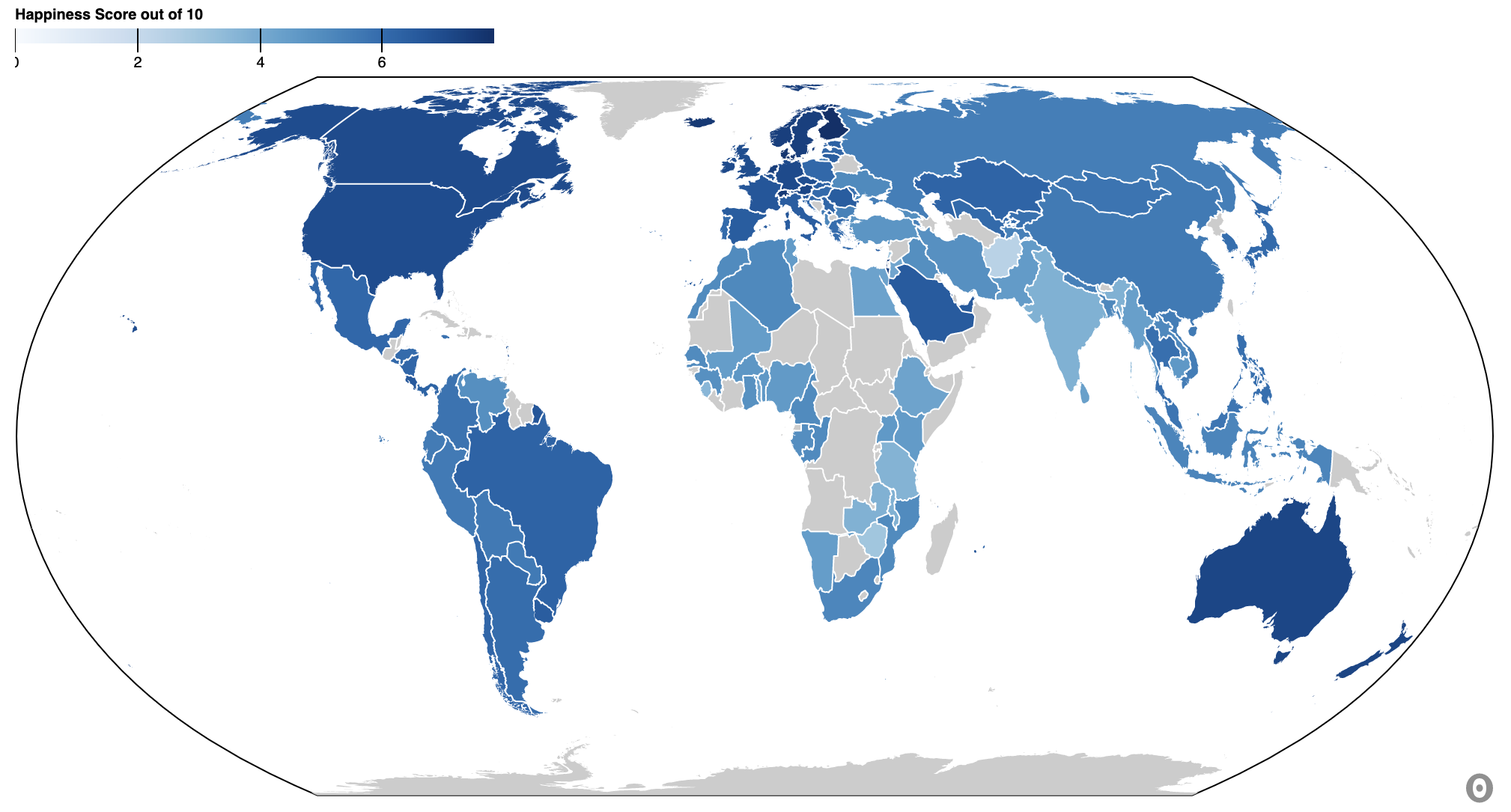
World Choropleth Map
Set Up
Before Starting make sure to have Observable-Jupyter and any other needed libraries installed in your local environment.
[1]:
from observable_jupyter import embed
import pandas as pd
import json
Load and Format Data
[2]:
Co2_df = pd.read_csv("Demo_data/2020_Co2_Emissions.csv", index_col = None)
[3]:
Co2_df.head()
[3]:
| Entity | Code | Year | Annual CO2 emissions (zero filled) | |
|---|---|---|---|---|
| 0 | Afghanistan | AFG | 2020 | 12160286 |
| 1 | Albania | ALB | 2020 | 4534673 |
| 2 | Algeria | DZA | 2020 | 154995460 |
| 3 | Andorra | AND | 2020 | 466294 |
| 4 | Angola | AGO | 2020 | 22198161 |
The following block of code structures the data into a format accepted by Observable.
[4]:
result = Co2_df.to_json(orient="records")
parsed = json.loads(result)
data = json.dumps(parsed, indent=4)
Formated_Data = json.loads(data)
Embed your data into the visualization
The World Choropleth Map is made up of two cells:
key_2 : acts as a legend for the map.
chart_2 : contains the map.
To make your visualization work you will need to access the input variables. In this visualization we have five variables that you can modify.
csv_data : set csv_data equal to your structured data.
feature : feature will be the equal to the column containing unique map entities.
quantitative_value : set equal to the column pertaining to the quantitative value you want to visualize.
color : Color ranges from 0-5 and gives you different color palets.
title : Title defines the title on the key
[5]:
embed(
    '@rstorni/choropleth-world-demo',
    cells=["chart_2", "key_2"],
    inputs = {
        'csv_data' : Formated_Data,
        'feature' : "Entity",
        'quantitative_value' : "Annual CO2 emissions (zero filled)",
        'color' : 5,
        'Title' : 'Co2 emissions per country'
    }
)